Overview
Typically when designing optical systems, engineers rely on ray tracing to calculate the paths and phases of light inside of a system. This method ignores much of the wave nature of the light except for the frequency or wavelength properties. Polarization ray tracing aims to extend these methods by also including the effects of the waves geometry (polarization), in the ray trace.

Since light is a transverse wave it is driven forward by an oscillating electric (and magnetic) field. This field can move in the vertical direction, horizontal direction, or at any angle in between. The electric field can even oscillate in a circular pattern if the movement in the x and y directions are out of sync. The orientation and phase of the electric field oscillation is the light's polarization. This example will go through the methodology and importance of polarization in optical design.
Jones Matrix Calculus
We think that the concept of polarized light was first observed in 1669 (Erasmus Bartholinus, Dutch) by viewing double refraction through a calcite crystal. For the next 200 + years much more observations and mathematical descriptions of polarized light were made (Malus Law ~1808, Fresnel Coefficients ~1830), but it was not until 1941, that a rigorous description of the phenomena was conceived by R.C. Jones. The American born physicists, methodology (now known as Jones Calculus), describes polarized light with a complex two dimensional Jones vector, and describes the optical interaction of polarized light with optical components using a complex 2 by 2 Jones Matrix. Jones vectors describe the electric field amplitude and phase and Jones matrices describe how materials/optical components will change the lights amplitude and phase.
$$Jones Vector \begin{pmatrix}J_{x}\\J_{y}\end{pmatrix}$$ $$Jones Matrix \begin{pmatrix}J_{xx} & J_{yx} \\J_{xy} & J_{yy} \end{pmatrix}$$ $$Polarized Interaction \begin{pmatrix}J_{xx} & J_{yx} \\J_{xy} & J_{yy} \end{pmatrix} \cdot \begin{pmatrix}J_{x_{in}}\\J_{y_{in}}\end{pmatrix} = \begin{pmatrix}J_{x_{out}}\\J_{y_{out}}\end{pmatrix}$$
This calculus describes fully polarized coherent light and how it interacts with materials. A little later on (1943), Hans Mueller, developed an overlapping calculus to describe incoherent interactions in terms of intensities. Though both methods should be used to get the complete polarization picture, we will focus on extending the Jones Calculus methods, so that they can be used during ray tracing.
Fresnel Aberrations
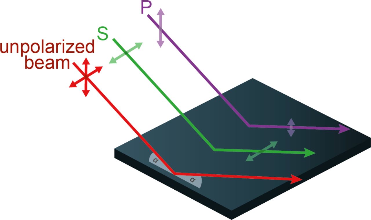
The amount of light that reflects and refracts off an optical interface, depends on the incident polarization and can be calculated using the Fresnel Equations (~1830, Augustin-Jean Fresnel, French). The equations divide the incident wave into two components, call S and P polarizations. Where the S-polarized direction is perpendicular to the plane of refraction, and the P-polarized direction is parallel to the plane of refraction.
These equations only depend on the incident ray angle and the refractive index on either side of the interface. All of these values are readily available during a ray trace.
$$ r_{s} = {n_{1} Cos\theta_{i} - n_{2} Cos\theta_{t} \over n_{1} Cos\theta_{i} + n_{2} Cos\theta_{t}} $$ $$ r_{p} = {n_{2} Cos\theta_{i} - n_{1} Cos\theta_{t} \over n_{2} Cos\theta_{i} + n_{1} Cos\theta_{t}} $$ $$ t_{s} = {2 n_{1} Cos\theta_{i} \over n_{1} Cos\theta_{i} + n_{2} Cos\theta_{t}} $$ $$ t_{p} = {2 n_{1} Cos\theta_{i} \over n_{2} Cos\theta_{i} + n_{1} Cos\theta_{t}} $$
Commonly, in optical systems there are air-glass interactions for refractive (lens) surfaces and air-aluminum interactions for reflective (mirror) surfaces. The corresponding Fresnel Coefficients as a function of the angle of incidence (AOI) are plotted bellow.
The Fresnel coefficients can be combined with the Jones Calculus to create a description for how an optical surface in an optical system will affect the polarization of the light propagating through the system.
$$JonesMatrix_{trans}= \begin{pmatrix}t_{s} & 0 \\0 & t_{p} \end{pmatrix}$$ $$JonesMatrix_{refl} = \begin{pmatrix}r_{s} & 0 \\0 & -1 \times r_{p} \end{pmatrix}$$
Though these Jones matrices will describe the optical polarization effects, they are somewhat limited in their applications to polarized ray tracing. This is because the Jones vector describes the electric field in terms of an x and y component. This has the implicit assumption that the light is propagating in the z-direction. Since one of the main goals of ray tracing is to calculate the change in propagation direction due to optical interactions, this formulation is clearly inadequate. To apply this methodology to three-D ray tracing, one must extend the Jones matrix into a three-D version.
Polarization Ray Trace (PRT) Matrix
The Jones matrix can be extended into three dimensions by calculating the directions of the propagation vector, s-polarization direction, p-polarization direction, before the interface ($k_{in}$, $s_{in}$, $p_{in}$) and after the interface ($k_{out}, s_{out}, p_{out}$), and preforming a local to global transformation.
$$PRT = O_{out} \cdot J \cdot O^{-1}_{in}$$ $$PRT = \begin{pmatrix}s_{x_{out}} & p_{x_{out}} & k_{x_{out}} \\s_{y_{out}} & p_{y_{out}} & k_{y_{out}}\\ s_{z_{out}} & p_{z_{out}} & k_{z_{out}}\end{pmatrix} \cdot \begin{pmatrix}S_{fresnel} & 0 & 0\\0 & P_{fresnel} & 0 \\ 0 & 0 & 1\end{pmatrix} \cdot \begin{pmatrix}s_{x_{in}} & s_{y_{in}} & s_{z_{in}} \\ p_{x_{in}} & p_{y_{in}} & p_{z_{in}} \\ k_{x_{in}} & k_{y_{in}} & k_{z_{in}} \end{pmatrix} $$
This method, takes the Jones matrix in local s-p space and transforms it into the global coordinate system, such that the resulting PRT matrix describes the polarized effects of the surface as well as the geometrical change in the ray propagation direction, and s and p polarization directions. The PRT matrices at each surface can then be multiplied together to represent the total polarization effects along a given ray path.
$$PRT_{total} = \prod_{surf=N,-1}^{1} PRT_n = P_N \cdot P_{N-1} ... \cdot P_2 \cdot P_1$$
Optical System Polarization Ray Trace Example
To illustrate the effectiveness of the above algorithm, lets run a polarization analysis on a simple optical system, and calculate how the optical surfaces will change the input polarization. The optical system will comprise of two refractive glass surfaces, defining a plano-convex lens, and an aluminum fold mirror that will redirect the light beam by 90 degrees into the detector.
A collimated ray set will be traced through the system and come to focus at the detector. This configuration will demonstrate how both refractive dielectric surfaces, a reflective metal surfaces, with a complex valued refractive index will affect polarized light.
System Polarization Analysis
Two quantities that are very important for optical designers to understand are diattenuation and retardance. These values will describe the polarization aberrations of the system. Polarization aberrations are polarization dependent deviations in both amplitude and phase from an ideal wave front. The diattenuation will describe the amplitude deviation and is defined as follows:
$$Diattenuation = {T_{max} - T_{min} \over T_{max} - T_{min}}$$
Where $T_{max}$ is the maximum transmission and $T_{min}$ is the minimum transmission. The retardance will describe the polarization-based phase dependence and is defined as follows:
$$Retardance = arg(\lambda_1) - arg(\lambda_2)$$
Where $\lambda_1$ is the first eigen polarization value and $\lambda_2$ is the second eigen polarization mode. *Note this definition assumes that the eigen polarization states are perpendicular.
To analyze this system the optical engineer will need to trace a grid of rays through the system. At each surface a PRT matrix will be used to calculate the surface polarization effects. Once the ray reaches the detector, all the individual surface PRT matrices can be multiplied together to calculate the polarization effects along the entire ray path. Then, the eigen values of the $PRT_{total}$ matrix, can be calculated. Since it is a 3 by 3 matrix, there will be three eigen values. By definition of the PRT matrix one of the eigen values will be 1. This corresponds to the propagation direction eigen value, which must be unity. The other two eigen values will most likely be complex, and the difference in phase between the eigen values will calculate the retardance. The maximum and minimum transmission values used to calculate the diattenuation can be ascertained by taking the absolute square of the eigen values.
Diattenuation due to Fresnel coefficients at each surface of the optical system
Total ray path diattenuation due to Fresnel coefficients at each surface of the optical system
Retardance due to Fresnel coefficients at each surface of the optical system
Total retardance due to Fresnel coefficients at each surface of the optical system
Effects on the electric field
Horizontal Input Polarization
Vertical Input Polarization
45 Degree Input Polarization
General Principals of Fresnel Aberrations
- There will be no polarization aberrations at normal incidence
- The retardance and diattenuation will increase with the angle of incidence
- The larger the numerical aperture the more retardance and diattenuation variation
- If either material at the optical interface has a complex valued refractive index, then there will be retardance
- There will be no retardance at a dielectric interface (i.e. air-glass)
- The larger the difference in refractive index values on either side of the interface, the larger the retardance will be
- Thin film coatings will generally decrease the diattenuation because they will increase both $r_s$ and $r_p$ or $t_s$ and $t_p$
- Thin film coatings (even if it is dielectric), will generally increase the retardance due to the interference effects